ProjectFEA
The goal of the project is to build an open source General Finite Element Library with easily defined weak forms.
 The basic inputs is a .msh file generated by Gmsh, a free 3D finite element mesh generator.
The weak form of can be easily declared in small class blocks within the main.cpp itself.
All boundary conditions, Neumann as well as Dirichlet boundary conditions can be delared within the main file.
The Nodes for Nuemann and Dirichlet boundary conditions are detected on the nodes declared as ‘Physical Groups’ in gmsh file. ProjectFEA consists of mostly just header files. Hence you will need to include the whole folder of ProjectFEA/Cpp folder within your source directory.
A Few Examples.
A few examples and gmsh files have been provided.
The included example source codes are, Poisson.cpp, ElasticityExample.cpp and OneElmntVrfy.cpp
You can run the Poisson example by running,
./Poisson <.msh file> <dimension of the Domain>
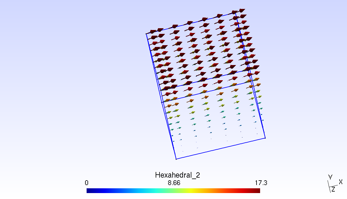
The .msh file “SampleGmsh/Hexahadral_2.msh” can be used for testing this example. Hence your input will be
./Poisson SampleGmsh/Hexahadral_2.msh 3
Similary ElasticityExample.cpp can be testing by running,
./ElasticityEx <.msh file> <dimension of the Domain>
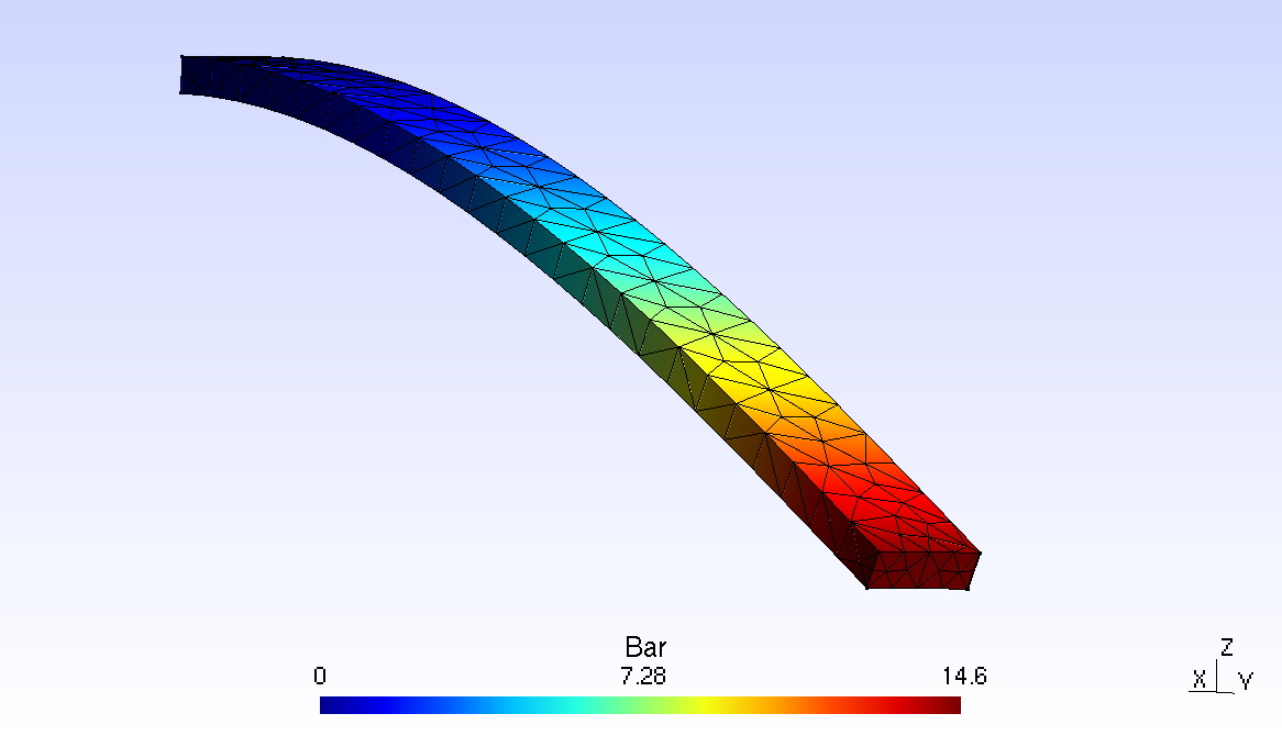
The .msh file “SampleGmsh/Bar.msh” or “SampleGmsh/Bar2.msh” can be used for testing this example. Hence your input will be
./ElasticityEx SampleGmsh/Bar.msh 3
or
./ElasticityEx SampleGmsh/Bar2.msh 3
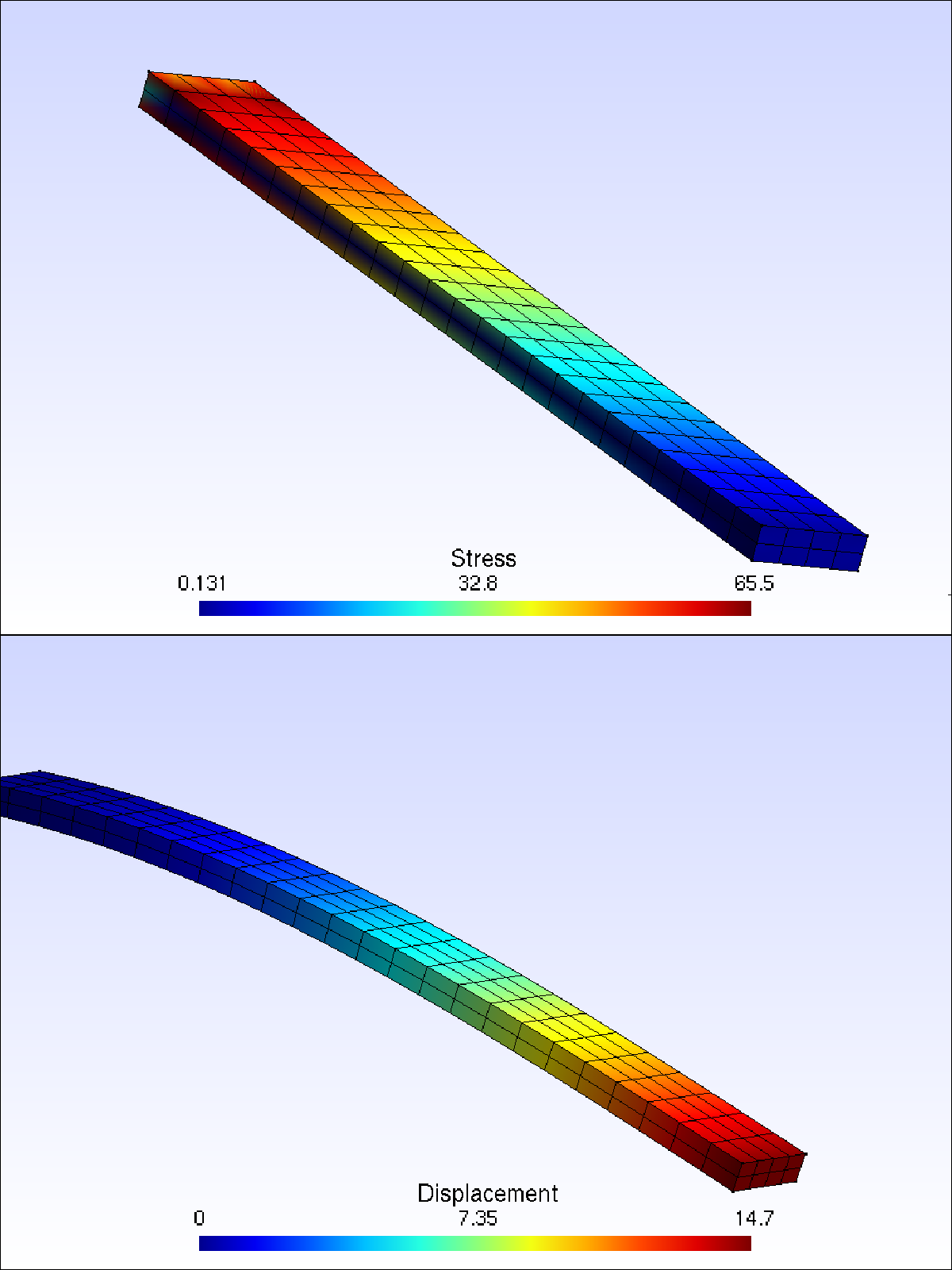
In case of the Bar example, a case of cantilever beam is tested, where a force of 4kN is applied at the end of a (2000mm x 200mm x 60mm) bar with a fixed end at the other side. The force is applied on the surface (200mm x 60mm). Young’s modulus is supposed 200 Gpa.
By using formula delta_L =Pl^3/(3EI) we get 14.8mm deflection.
The finite element converges to that solution as the order of the elements and the number of nodes are increased.
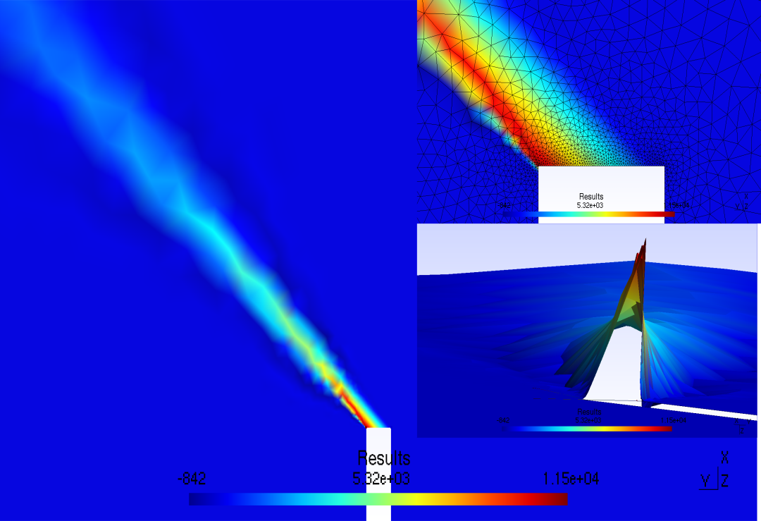
or Advection-Diffusion can be tried by running
./DiffusionEx SampleGmsh/Chimney.msh 2
or the Dynamic Heat Diffusion Problem can be tried by by running
./DynamicHeatDiff SampleGmsh/Rod.msh 3
or the Dynamic Vibration Problem can be tried by running
./ElasticVibration SampleGmsh/ForkLift.msh 3
One Click Download and Compilation
If you are using a Debian based Linux distribution (Ubuntu, Mint, Debian, SparkyLinux etc..), then you can try this one file download and compilation. This file downloads the requisite files, compiles them and even runs the OneElmntVrfy file to check that everything is running fine. You may download the file here….
How to Compile.
Before starting, in your Linux installation, make sure you at least have the following packages installed.
(include the dev package for Ubuntu/ Debian based distributions)
Armadillo
Blas
Lapack
SuperLU
To compile the code, you need to first download the latest Gmsh source code from gmsh.info/ and compile it.
You can also clone it by,
git clone https://gitlab.onelab.info/gmsh/gmsh.git
The Branch currently used by ProjectFEA is gmsh_4_4_1.
You can set it by typing
git checkout gmsh_4_4_1
Type the following in your Gmsh build directory. This will build a static library of Gmsh.
cmake -DDEFAULT=1 -DENABLE_BUILD_LIB=1 -DCMAKE_CXX_COMPILER=g++ -DCMAKE_CC_COMPILER=gcc <path gmsh source directory>
make lib
Clone the ProjectFEA Library by typing
git clone https://github.com/samadritakarmakar/Project-FEA.git
Copy the libgmsh.a file generated earlier to the folder ProjectFEA/Cpp/libGmshReader/GmshApi/
The go to your build directory and type
cmake -DCMAKE_CXX_COMPILER=g++ -DCMAKE_CC_COMPILER=gcc <path to source directory>
make
How to Use. (Still being Written)
To understand on how to use the library you should have some understanding of C++, Armadillo C++ library and Finite Element Methods, specially on how to derive weak forms.
Armadillo library is used in ProjectFEA for Matrix manipulations. Armadillo uses syntax that is very similar to Matlab/Octave. You can read more about the Armadillo project and it’s documentation here.
Before going forward, some understanding of the file structure of the Library is needed.
ProjectFEA -> _Main Project Directory._
├── Cpp -> _All C++ related files are here._
│ ├── armadillo -> _Project FEA depends on armadillo library for matrix manipulations._
│ ├── BaseGeom -> _Contains .geo files of one element domain. Lets ProjectFEA know how gmsh numbers it’s nodes in reference elements._
│ ├── DirichletBC -> _Contains files that are responsible for applying Dirichlet Boundary conditions._
│ ├── FEMtools -> _Contains some simple tools responsible for loading the right gauss file and manipulating the row/column position of data as per node position._
│ ├── GaussData -> _Contains text files having Gauss points and weights._
│ ├── GmshWriter -> _Sends post-process data back to Gmsh API to generate post-processing files._
│ ├── Integrator -> _Contains files that are responsible to integrate over the element (Local Integrator) and files responsible for global matrix assembly (System Assembler)._
│ ├── libGmshReader -> _Contains files that are responsible for reading data in Gmsh files._
│ ├── Math -> _Contains a few math functions._
│ ├── Models -> _Weak forms and other formulations of models are to be coded here for easy reuse._
│ ├── OneElmntGeom -> _Sample One Element geometry files are here to provide for testing algorithms._
│ ├── Pics -> _Pictures of Simulations are saved here._
│ ├── ProjectJacobian -> _This has files to calculate Jacobian of vectors._
│ ├── SampleGmsh -> _Contains Sample geometry and mesh files for Testing._
│ ├── ShapeFunction -> _Contains files responsible for generation of Shape Functions._
│ ├── TestAndTrialFunction -> _Contains the Form Class that is responsible for easy declaration of weak forms and all the different kinds of Test and Trial Function codes._
│ └── Variable -> _Contains files that allow for the easy declaration of array type data._
├── Octave -> _Contains old octave/Matlab files that were once used as a proof of concept._
So let us start with the definition of a weak form in ProjectFEA. (Poisson Single Thread Example)
If you open the file Project-FEA/Cpp/Integrator/ LocalIntegration.hpp you will see at least three different virtual functions defined. They are “weak_form”, “weak_form_vector” or “scalar_integration”.
- “weak_form” is to be used for definition of the part of weak form that result in matrices to being formed. Such as the stiffness matrix ‘A’ in the equation ‘[A]{x}={b}’.
- “weak_form_vector” is to be used for definition of the part of weak form that result in vectors to being formed. Such as the vector ‘b’ in the equation ‘[A]{x}={b}’.
- “scalar_integration” can be used to find out some scalar properties of the element. For example, the volume of an element can be found by integrating over dX.
For defining the weak form, a new class has to be defined which inherits the class LocalIntegrator defined in LocalIntegration.hpp.
To use any of these functions, it is advised to head over to the file LocalIntegration.hpp and copy the function to the class of your definition without the virtual keyword.
You may now refer to the example of Poisson.cpp which in this case is a single thread definition and is easy to understand for starting with ProjectFEA. Poisson equation has the weak form given below, if it has a source term b and well as a Neumann Boundary Condition where the flux is equal to the vector t.

The Left hand side of this equation may represented by the following code as seen in Poisson.cpp
        /// A new Model is defined here. This weak form is integrated over each element.
        /// The Virtual 'weak_form' function defined in 'LocalIntegrator' is overloaded during runtime.
        class new_LocalIntegrator: public LocalIntegrator<TrialFunction>
        {
        public:
                new_LocalIntegrator(Form<TrialFunction>& a, TrialFunction& u, TestFunctionGalerkin<TrialFunction>& v):
                LocalIntegrator (a,u,v)
                {
                }
                sp_mat weak_form(Form<TrialFunction>& a, TrialFunction& u, TestFunctionGalerkin<TrialFunction>& v)
                {
                    return a.inner(a.grad(v),a.grad(u))*a.dX(u);
                }
        };
The source term may be defined as,
        /// The Virtual 'weak_form_vector' function defined in 'LocalIntegrator' is overloaded during runtime.
        class new_LocalIntegrator2: public LocalIntegrator<TrialFunction>
        {
        public:
                new_LocalIntegrator2(Form<TrialFunction>& a, TrialFunction& u, TestFunctionGalerkin<TrialFunction>& v):
                LocalIntegrator (a,u,v)
                {
                }
                mat weak_form_vector(Form<TrialFunction>& a, TrialFunction& u, TestFunctionGalerkin<TrialFunction>& v)
                {
                vec b;
                b<<0<<endr<<0<<endr<<0<<endr;
                return a.dot(v,b)*a.dX(u);
                }
        };
And the flux over the Neumann Boundary can be defined as,
        /// The Virtual 'weak_form_vector' function defined in 'LocalIntegrator' is overloaded during runtime.
        class new_Neu_Surf_LclIntgrtr: public LocalIntegrator <TrialFunctionNeumannSurface>
        {
        public:
            new_Neu_Surf_LclIntgrtr(Form<TrialFunctionNeumannSurface>& a, TrialFunctionNeumannSurface& u,
            TestFunctionGalerkin<TrialFunctionNeumannSurface>& v):
            LocalIntegrator (a,u,v)
            {
            }

            mat weak_form_vector(Form<TrialFunctionNeumannSurface>& a, TrialFunctionNeumannSurface& u,
            TestFunctionGalerkin<TrialFunctionNeumannSurface>& v)
            {
                vec vctr={1,1,1};
                return a.dot(v,vctr)*a.dS(u);
            }
        };
The Dirichlet Boundary Condition can vary according to the positon of the node in the domain. This variation in the Dirichlet obundary condition is acheived in ProjectFEA by definiting a virtual function Eval in the class Expression that is defined in the file Project-FEA/Cpp/DirichletBC/Expression.hpp. A new class has to be defined which ineherits the Expression class and overloads its virtual function Eval to apply boundary condition. Within the class DirichletBC defined in Project-FEA/Cpp/DirichletBC/DirichletBC.hpp the vector of the current postion of the node is passed to the function Eval, which may be used to vary the Dirichlet Boundary according to the node positon.
        ///This class over here through its overloaded virtual function declares the values of Dirichlet Nodes.
        /// The virtual function 'Eval' is evaluated at each node to find the value of Dirichlet Condition at that node.
        class DeclaredExprssn : public Expression
        {
        public:
            DeclaredExprssn (int vectorLevel): Expression (vectorLevel)
            {
            }
            vec Eval(vec& x)
            {
                vec value={0,0,0};
                return value;
            }
        };
Once the weak forms are defined, you may start to write the main() file.
You can start by telling ProjectFEA the mesh file that you wish to use. For example,
    int main()
    {
        int Dimension=3;
        libGmshReader::MeshReader Mesh("SampleGmsh/Hexahedral_1.msh", Dimension);
This will make ProjectFEA read the given mesh and store it’s relevant data in Mesh. The Dimension integer variable is the dimension of the domain, which in this case is 3.
Next we look at how the matrices are calculated. For that, you must first know what is the degree of freedom per node of the quantity that has to be evaluated. In ProjectFEA this degree of freedom has been named as vectorLevel. Since Poisson equation is quite flexible and the quantity may be a scalar or a vector, here we have considered a vector with a degree of Freedom 3.
int vectorLevel=3;
Then, the Trial Function has to be defined with the declared mesh variable and the vectorLevel.
    /// Declaration of Quantity to be Calculated.
    TrialFunction u(Mesh,vectorLevel);
Next the TestFunction has to be defined. ProjectFEA provides for Galerkin Type Test Functions to be declared. That may be defined as the following.
TestFunctionGalerkin<TrialFunction> v(u);
The file Project-FEA/Cpp/TestAndTrialFunction/Form.hpp is the interface that makes it easy to define weak forms, keeps track of the element that is being integrated and also the Gauss point at which the current integration iteration is.
Form<TrialFunction> a;
ProjectFEA needs to know which class definition has the weak form which has to be evaluated. So an instance of the newly defined class defining the left hand side of the weak form is declared.
new_LocalIntegrator lcl_intgrt(a,u,v);
Now, you need to tell ProjectFEA the class name that you have defined, the kind of Function it is (in this case TrialFunction) and the pass it the instances of Form, TrialFunction and TestFunctionGalerkin as shown below. SystemAssembler is a class defined in Project-FEA/Cpp/Integrator/SystemAssembly.hpp that is responsible for this.
SystemAssembler<new_LocalIntegrator, TrialFunction> systmAssmbly(a,u,v);
In Finite Element Method, the stiffness matrices are generally sparse matrices. ProjectFEA tries to take advantage of this fact. Using the Armadillo API, a sparse matrix is defined and is sent back to the SystemAssembler to set it’s size.
    sp_mat A;
    systmAssmbly.SetMatrixSize(A);
Now, the matrix is ready for assembly and is sent to the RunSystemAssembly function within the SystemAssembler class for creating the Global matrix.
systmAssmbly.RunSystemAssembly(lcl_intgrt, A);
Now that the matrix A is ready.
Next, the vector b has to be assembled. Similar to what we did for the matrix A, vector b can be assembled. Below the source term is integrated over.
    Form<TrialFunction> a2;
    new_LocalIntegrator2 lcl_intgrt2(a2,u,v);
    SystemAssembler<new_LocalIntegrator2, TrialFunction> systmAssmbly2(a2,u,v);
    mat b;
    systmAssmbly2.SetVectorSize(b);
    systmAssmbly2.RunSystemAssemblyVector(lcl_intgrt2, b);
In ProjectFEA, once a matrix or a vector is declared for Global assembly, every System Assembly only adds to the current Matrix or Vector. Using this philosophy, we add the Neumann Boundary equation, i.e., the last term in the given weak form equation. That is done by the given next few lines.
    Form<TrialFunctionNeumannSurface> a3;
    TrialFunctionNeumannSurface u_surf(u,0);
    TestFunctionGalerkin<TrialFunctionNeumannSurface> v_surf(u_surf);
    new_Neu_Surf_LclIntgrtr lclintgtr3(a3,u_surf, v_surf);
    SystemAssembler<new_Neu_Surf_LclIntgrtr, TrialFunctionNeumannSurface> systmAssmbly3(a3, u_surf, v_surf);
    systmAssmbly3.RunSystemAssemblyVector(lclintgtr3, b);
The matrix A and the vector b is now ready for application of Dirichlet Boundary Condition.
The way of applying the Dirichlet Boundary Condition has quite some similarities with way weak forms are evaluated. If suppose there are 3 degrees of freedom per node, then the user may or not want to apply the Boundary condition on all the 3 degrees of freedom. This can be acheived by setting a umat type matrix. If the value for a certain degree of freedom is zero(0) then the Dirichlet Boundary is not applied for that degree of freedom. Here the Boundary condition is appleid for all the nodes, hence the variable is defined as given below.
umat boolDiricletNodes={1,1,1};
Next an instance of the class DirichletBC is delared.
In the first argument passed for the declaration of the instance ProjectFEA needs to know where the nodes lie. If suppose the nodes lie on volume, then passing an instance TrialFunction is sufficient. If it lies on a surface, then an instance of TrialFunctionNeumannSurface has to be passed and in case of a line an instance of TrialFunctionNeumannLine has to be passed.
For the second argument the index of the Physical Group has to be defined. It should be noted that index of the Physical Group number is not the same as the Group Number defined in Gmsh but rather similar to the order in which the physical groups have been defined. If it was the 1st physical group to be defined, then the index would be 0, if 2nd in order, then 1 and so on.
Finally, the last argument is for the umat of the Dirichlet Nodes where boundary conditions would have to be applied, as explained earlier.
DirichletBC DrchltBC(u_surf,1, boolDiricletNodes);
An instance of the newly declared expression is defined and is passed on the the function SetDirichletBCExpression defined in the class DirichletBC from the file, Project-FEA/Cpp/DirichletBC/DirichletBC.hpp. After that, the Boundary Condition is applied using the function ApplyBC from the same class.
    DeclaredExprssn Dirich(vectorLevel);
    DrchltBC.SetDirichletBCExpression(Dirich);
    DrchltBC.ApplyBC(A,b);
The matrix A and the vector are now ready to be solved. Armadillo’s sparse matrix solver can be used for this purpose and we can use the [spsolve] function for this and we have two alternatives for this.
either,
mat X=spsolve(A,b);
or,
    mat X;
    spsolve(X, A, b);
The second option is a better option, but it does not stop the program if the system of equation [A]{X}={b} has no solution.
Finally, the solution can be be sent back to the Gmsh API to write an output file. GmshWriter class defined in the file Project-FEA/Cpp/GmshWriter/GmshWriter.hpp can be used to do this. First the TrialFunction is passed and then the name of the output file is passed. Then the function WriteToGmsh defined in the class GmshWriter is used to write the solution matrix to the output file.
    GmshWriter Write(u, "poisson.pos");
    Write.WriteToGmsh(X);